Aerospace Micro-Lesson #98
In This Section
Iteration and Chaos in Mathematics
Iteration—doing the same thing over and over again—sounds like a very boring proposition. But it can produce results of great beauty and of literally infinite complexity. The mathematical field of chaos theory, which came into vogue in the 1980s, is based on repeating the same operation infinitely many times, each time using the output of the previous operation as input to the next operation. This lesson emphasizes the simplicity of iterative processes and the beauty and grandeur of the results that they give.
Common Core State Standards (CCSS): Math:
- Standard for Mathematical Practice: Reason abstractly and quantitatively.
GRADES K–2
We learn to count in one-to-one correspondence in kindergarten, but that is not the only way to count. We also learn skip counting, to count by 2s or 5s or 10s, for instance. But there are even more interesting ways to count. The Fibonacci Sequence is one of those ways. In this way of counting we start with “0, 1” and then each number after that is the sum of the two numbers that precede it. So the sequence begins with “0, 1, 1, 2, 3, 5, 8, 13…” and can go on to infinity.
The number series was published in a book called Liber Abaci by a man known as Fibonacci in the 13th century, but it had been known even before then. Since he wrote about it, the sequence is named for him. The Fibonacci Spiral can be built from shapes based on numbers in the sequence, such as using tiles to fill a space in increasing squares, then tracing outward from that first tile and around the outer corners of each successively larger square area.
Think of the places in nature where such spirals exist - in the curves of seashells, the shape of galaxies, the arrangement of florets on a pinecone, or the petals on a flower - and those are just a few.
To introduce the idea that math concepts really do apply to real life in all sorts of unexpected ways, you might like to read The Math Curse by Jon Sceiszka and Lane Smith to your class. Then see if they can find similar examples throughout the day.
For your own inspiration, consider watching this TED Talk on The Magic of Fibonaccai Numbers.
GRADES 3–5
Pick a number. Any number. (Well, okay, it has to be a positive whole number—a counting number.) If it is even, divide it by two. If it is odd, multiply it by three and add one. You get a new number. Repeat the operation—dividing by two or else multiplying by three and adding one—on the new number. Keep doing it over and over again. Eventually you will get into a cycle of numbers: 4, 2, 1, 4, 2, 1, 4, 2, 1, … .
If you start with another counting number, you will go through a different sequence of numbers, but eventually you will wind up at the same cycle: 4, 2, 1, 4, 2, 1, and so on.
Question: Is there a number that you can start at that does NOT land you in that same cycle? Nobody knows. Literally, nobody knows. This is an unsolved problem in mathematics. The Collatz Conjecture states that if you repeat this operation enough times starting with any number, you will eventually end up at that cycle, but it is just a conjecture. Nobody has proven it right; nobody has proven it wrong. A great mathematician, Paul Erdös (pronounced “Air-dish”), once said that “Mathematics is not yet ready for such problems.” John Horton Conway, another great mathematician, considered a more general version of the problem and proved that the more general version cannot be proven or disproven. If nothing else, this shows just how close at hand in mathematics the unknown can lurk.
If your students want to try their hands at generating sequences starting from various numbers, feel free to encourage them. It has been demonstrated that a sequence starting with any number less than about 5.48×10¹⁸ will end at 1, so there is not much chance that your students will find a counterexample. You may also want to encourage your students to continue their studies in mathematics until they can analyze this problem more generally.
GRADES 6-8
Start with a line segment. Take out the middle third of the line segment and replace it with two line segments of the same length, forming an equilateral triangle with the line segment that was removed. Then repeat the process for each of the four line segments. After these two operations you have something that looks like this (the red line segments have just been put into the figure and the blue lone segments are there from before):
(the red line segments have just been put into the figure and the blue line segments are there from before).
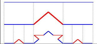
Now do it again and again and again. Eventually you have something that looks like this:
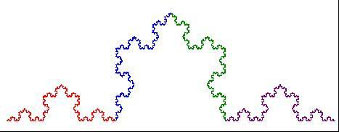
How long is this curve? Well, if your first straight line was one foot long, then your second figure (with four line segments, each one third of a foot long) was 4/3 feet long. Then your third figure (with 16 line segments, each one ninth of a foot long) was 16/9 feet long. Each time you take out the middle third of your line segment and replace it with two more just like it, you are multiplying the length of the curve by 4/3. If you do this infinitely many times, then the length of the curve becomes

which, after infinitely many multiplications, is infinitely large. Think about that: a curve of infinite length is contained between two endpoints a foot apart.
Another feature of the Koch curve is that if you zoom in on any part of it, that part looks exactly like the whole curve. (Wikipedia has an animation which shows this very well.) This property is what makes a fractal a fractal: any part of it is similar to the whole. Contrast this with zooming in on a circle, where a circular segment looks more and more like a straight line the closer you get in to it. Or you can contrast this with a square, where you see one thing if you zoom in on a corner and another thing if you zoom in on an edge.
Fractals have a strange beauty about them. A possible reason for this is that in many ways, they mirror nature and nature is intrinsically beautiful. A tree trunk splits up into limbs, which split into smaller branches, which split into twigs, in the same way that a fractal repeats itself on ever smaller scales. Waves in the ocean form into larger swells and have smaller wavelets on top of them. Clouds have large billows whose surfaces have smaller puffs which are made up of ever smaller details. Fractals imitate these repetitions on ever-smaller scales, extending the repetition down to infinitesimal scales.
If you want to analyze the Collatz Conjecture sequence described in the Grades 3-5 lesson, here are a couple of pointers. Consider the odd numbers in the sequence. For each of these odd numbers, you will multiply it by three and add one, making the next number an even number. Now consider these even numbers. Half the time the next even number will be divisible by two but not by four. One quarter of the time it will be divisible by four but not by eight. One eighth of the time it will be divisible by eight but not by 16. This continues as far as you would like to take it. The next odd number, then, will be about 3/2 times the value of the current odd number half the time, 3/4 times the value a quarter of the time, 3/8 times the value one eighth of the time, and so on. Adding all these probabilities together gives a series:

A little arithmetic shows that this series adds up to one. This means that on average, the next odd number will be about the same as the present odd number. If the series added up to a number less than one, this would indicate that eventually the Collatz sequence would converge to a value of one. If the series added up to a number greater than one, this would indicate that the Collatz sequence would give ever larger numbers and increase without bound. But because the series adds up to exactly one, the Collatz sequence is balanced on the knife edge.
Mathematicians have generalized the Collatz sequence to consider dividing by a general number in the one case and multiplying by another general number and rounding up to the next multiple of the first number in the second case. The sequences created by these more general rules form various cycles.
GRADES 9-12
Consider a very simple nonlinear equation:

It defines a parabola which passes through the origin and has another zero at “x = a”. We can use it to generate a sequence of numbers:

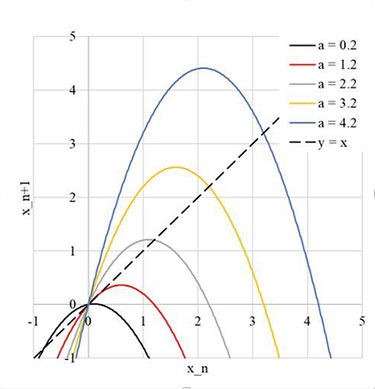
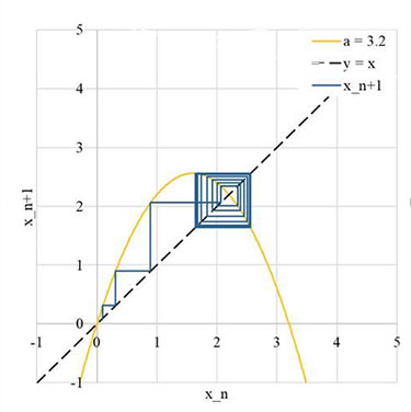
This is called the “Discrete Logistic Equation” and is used in modeling the growth of a population with limited resources. The factor “a” is the population’s growth rate and the quadratic term models the exhaustion of, for example, the food supply if the population is too great. (There is a continuous Logistic Equation, but its solution involves calculus and it is best reserved for college students.) One can graph the curves generated by various values of “a”, as is shown on the right. Creating the sequence using the formula can be thought of using the graph as finding a point on the curve for the appropriate value of “a” (this is equivalent to using the formula to calculate xn+1), then moving horizontally to the “y = x” line (this moves xn+1 to become the next xn), then moving vertically to the curve again (to calculate the next xn+1). On a graph, one generates something similar to the figure below. (*** Fix the wording as the pagination adjusts ***)
The obvious question is, what will happen to xn as “n” becomes arbitrarily large, if you start with x0 somewhere between 0 and a? (If you start the sequence with x0 outside that interval and with a positive a, the next term is negative and the sequence goes off to negative infinity. You can invite your students to figure out what happens if a is negative.)
There are four possibilities.
The first possibility is that xn will go toward negative infinity. If a is greater than 4, the top of the parabola is larger than a and the next horizontal move to the “y = x” line gives you a negative value for xn+1 on the next iteration. You can specify initial values for x0 which will prevent this from happening (such as x0 = a – 1), but most initial values for the sequence will cause the values to go toward negative infinity.
The second possibility is that xn will converge to a single value. If a is less than one, the sequence will converge at xn = 0; if a is between one and three, the sequence will converge at xn = a – 1. This happens when the slope of the parabola at the point where it crosses the “y = x” line is less than one.
The third possibility is more interesting: the sequence will converge to what is called an “n-cycle.” In an “n-cycle,” the value of x jumps back and forth in a repeating set of n different values. (The “n” here is different from the “n” that denotes the position of the term in the sequence.) This possibility is shown in the graph above, showing that for a = 3.2 the sequence xn converges to a 2-cycle. As a increases beyond three, the sequence converges first to a 2-cycle, then to a 4-cycle, then to an 8-cycle, and so on.
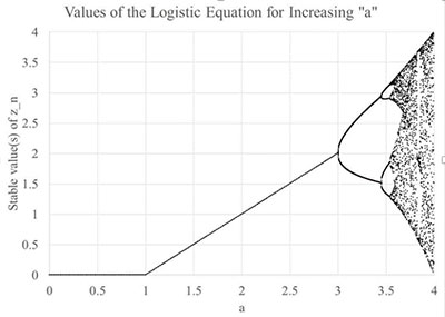
The fourth possibility is the most interesting: xn may jump around between an upper limit and a lower limit and never repeat itself. As a increases, the length of the n-cycle keeps doubling until eventually around a = 3.57 it becomes infinite. Above a = 3.57, for a random initial value x0, the numbers xn never repeat themselves but never go outside the interval from 0 to a. This behavior is called “chaos” and was first investigated by Mitch Feigenbaum for the Discrete Logistic Equation in the 1970s. If you have students with a mathematical bent, they write a program (or generate a spreadsheet) quite easily to model the behavior of this sequence. Failing that, Wolfram MathWorld has two very nifty demonstrations of how the sequence behaves for different values of “a”. The figure to the right shows the values of xn to which the sequence converges as “a” increases.
The essential features of chaotic behavior are that later values of a variable (such as the term in the sequence) depend on earlier values and that these later values are very sensitive to changes in the earlier values. This “sensitive dependence on initial conditions” is a hallmark of chaotic behavior.
That something as simple as a quadratic equation with a single free parameter can lead to chaotic behavior is startling. Research into chaotic behavior of systems is not difficult; one can do it with a little algebra.
What about a more general quadratic equation? It turns out that one can simplify most quadratics into the form analyzed here. We start with a completely general quadratic:

We have three free parameters here: A, B, and C. We scale and offset our “x” values (where we will specify the values of “p” and “q” later):

Putting this into our equation gives

We can specify


(note that being a quadratic, the latter equation doesn’t always have a solution) to get

where “a = B – 2 q”. Our three free parameters (A, B, and C) have been reduced to the single parameter “a”. In plain English, if somebody specifies A, B, and C, you can often calculate a “p” and “q” to reduce the equation to the form that was analyzed. The behavior of the equation in cases in which the quadratic equation for q does not have a solution is left as an exercise for your motivated students.
Sixty Years Ago in the Space Race:
